Formula based coloring

[InfaReQt]

Hello everyone,

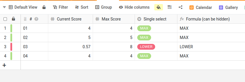
I’m currently working on implementing score comparisons in my setup. The idea is to highlight cells in green if the current score matches the maximum score, and in red if it doesn’t. To achieve this, I added an extra row with a formula that compares the values. Currently, it displays the current score only when it matches the max score; otherwise, it remains blank.

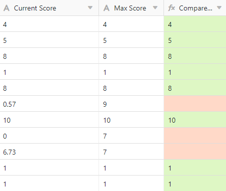
I then set up a coloring rule where cells turn green if they are not empty and red if they are. However, I would prefer the number to be visible even when it doesn’t match. The challenge is that altering the formula to display the number in such cases disrupts the coloring rules due to their limitations.

Is there a way to use formulas to apply cell colors based on specific conditions, even when the content is displayed?

Thanks in advance for your assistance!

[cdb]

Hey InfaReQt,
Color (Use rules) can not compare different columns. Therefore, I don’t see an easy solution, to show the value and use the coloring at the same time. As soon as you print also the lower numbers, the criteria for the color is gone.

I see the alternative, that you use a single select column and then color the row based on this single select column. The value of the single select column is set by an automation every time a number is entered. The automation watches the formula and sets the single select column.

[InfaReQt]

Thanks for the response
I’ll use this workaround for now, it’s not a big issue luckily